A first PyTorch test: I am a wizard

Following the quickstart tutorial on the PyTorch docs, I coded up a Google Colab notebook to test some simple machine learning frameworks on a relatively easy dataset, FashionMNIST. I did this in order to feel the power of machine learning in my hands, but also to take a look at the process of training a model.

For context, FashionMNIST consists of 28x28 grayscale images of clothing items, each of which fits in one of 10 categories of clothing. Therefore, the problem of understanding FashionMNIST is a classification problem.

I first used the prototypical example of a neural network: a multilayer perceptron, or MLP. The orignal specifications were a network with (784, 512, 512, 10) nodes per layer, respectively, as well as the following choices:

Activation function: ReLU
Loss function: Cross entropy (standard for classification)
Optimizer: Adam
Learning rate: 0.001

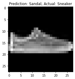
With 10 epochs of training on the learning data, this model attained an accuracy of 87.6%. Not too shabby. I had a bit of fun using MatPlotLib to see which examples the model got wrong.

wrong-prediction-haha

I soon discovered, however, that the number of interal nodes in this model was somewhat overkill. I eventually shrunk the model to (784, 64, 10), which still maintained an accuracy of 87.1%.

I also discovered that the initial 87.6% was apparently quite close to the ceiling for an MLP, since training for 10 more epochs only brought the accuracy to 87.8%. In fact, the diminishing returns began quite early on. Here’s a plot showing the change in accuracy over time:

accuracy-over-time

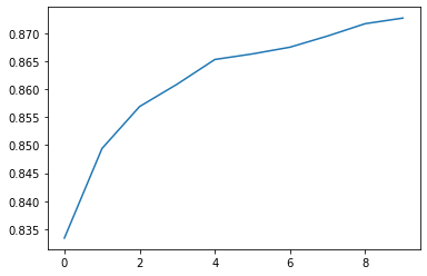
Note the x-axis. The first epoch alone managed to achieve an 83% accuracy. Of course, more accurate is better, but it would be ideal to somehow converge to 100%, or at least something above 88%.

Takeaways:

There are some “hard” examples in the dataset that for some reason require much more nuance to model than the rest of the data. Although some of the model’s mistakes would be obvious to a human, as the picture above, it was clear that some were legitimately difficult to tell apart. This would explain the 88% accuracy cap.
Conversely, there are a lot of “easy” examples. I never got an accuracy below 83%, except for when I forgot to restart the runtime and the model freaked out.
Although training for more epochs did not significantly increase the accuracy, it did decrease the total loss. This indicates that the model was getting more confident despite not getting better at the actual decision problem. (I’ve heard about this being a problem with overtraining!)
Simply adding more nodes/layers has diminishing returns in terms of better accuracy. To make substantial improvements, a new framework is required.

And that new framework is a convolutional neural network, or CNN, designed to encode 2D proximity data in a way that MLPs fail to do.

The layers I used were:

convolution with 16 channels of kernel size 5
ReLU
max pool with kernel size 2
convolution with 32 channels of kernel size 7
ReLU
max pool with kernel size 2
flatten (turn 2D data into 1D data)
linear (perceptron) to 10 outputs.

With just 10 epochs, this CNN achieved 90.7% accuracy! Even 5 epochs was enough to beat the MLP, achieving 88.5% accuracy. Definitely still not converging to 100%, but already an improvement.